R : A Simple Decision Tree and Random Forest Example

Decision trees are a popular tool in machine learning. They take a form of a tree with sequential questions which leads down a certain route to give an answer.

Tree models where the target variable can take a discrete values are called classification trees, whereas when target variable takes continuous values they are called regression trees.

The model takes the form “if this .. then that” conditions to arrive to a specific outcome. Tree depth is an important concept. This represents how many questions are asked before we reach our result.

Random forests are a collection of decision trees whose results are aggregated into one final result. They are a powerful tool due to their ability to limit over-fitting without substantially increasing error due to bias which is a common case when using decision trees.

Random forests are a collection of decision trees whose results are aggregated into one final result. They are a powerful tool due to their ability to limit over-fitting without substantially increasing error due to bias which is a common case when using decision trees.

We will apply both Decision trees and Random forests models to the famous “kyphosis” dataset. The objective is to determine important risk factors for kyphosis following surgery.

The data was collected on 83 patients undergoing corrective spinal surgery:

• Kyphosis : with the value “absent” or “present” indicating if a kyphosis was present after the operation.

• Age : the age in months

• Number : the number of vertebrae involved

• Start : the number of the first vertebra operated on

We will use R in this post, here is the Python version. So let´s start :).

Preparing the data

We will use the the “rpart” library, which includes our data and is used for recursive partitioning and regression trees.

library(rpart)
k_df = kyphosis

head(k_df)

Kyphosis	Age	Number	Start
absent	71	3	5
absent	158	3	14
present	128	4	5
absent	2	5	1
absent	1	4	15
absent	1	2	16

str(k_df)

'data.frame':	81 obs. of  4 variables:
 $ Kyphosis: Factor w/ 2 levels "absent","present": 1 1 2 1 1 1 1 1 1 2 ...
 $ Age     : int  71 158 128 2 1 1 61 37 113 59 ...
 $ Number  : int  3 3 4 5 4 2 2 3 2 6 ...
 $ Start   : int  5 14 5 1 15 16 17 16 16 12 ...

We can see that there are 2 missing from the count. It turns out that cases 15 and 28 were removed.

any(is.na(k_df))

FALSE

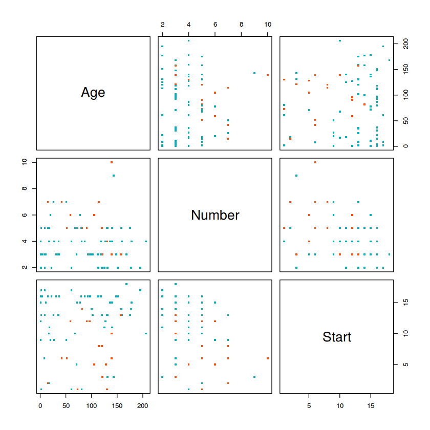
colors <- c("#00AFBB", "#FC4E07")
pairs(k_df[2:4],pch = 15,  cex = 0.6,
      col = colors[k_df$Kyphosis])

Decision Tree

tree_model <- rpart(Kyphosis ~ . , method='class', data= k_df)

# display cp table
printcp(tree_model)

Classification tree:
rpart(formula = Kyphosis ~ ., data = k_df, method = "class")

Variables actually used in tree construction:
[1] Age   Start

Root node error: 17/81 = 0.20988

n= 81

        CP nsplit rel error xerror    xstd
1 0.176471      0   1.00000 1.0000 0.21559
2 0.019608      1   0.82353 1.1176 0.22433
3 0.010000      4   0.76471 1.1176 0.22433

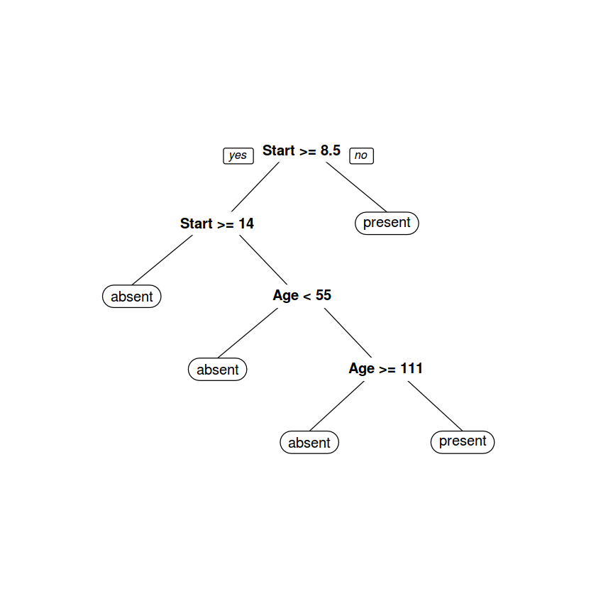
# We can plot the decision tree
# using "rpart.plot" library
# install.packages('rpart.plot')
library(rpart.plot)
prp(tree_model)

Random Forests

# we will import "randomForest" library
# install.packages('randomForest')
library(randomForest)

randomForest 4.6-12
Type rfNews() to see new features/changes/bug fixes.

rf_model <- randomForest(Kyphosis ~ .,   data=k_df)

# display the result
print(rf_model)

Call:
 randomForest(formula = Kyphosis ~ ., data = k_df)
               Type of random forest: classification
                     Number of trees: 500
No. of variables tried at each split: 1

        OOB estimate of  error rate: 20.99%
Confusion matrix:
        absent present class.error
absent      59       5   0.0781250
present     12       5   0.7058824

# how important is each of our predictors
importance(rf_model)

	MeanDecreaseGini
Age	8.497910
Number	5.455633
Start	10.189790