
R : An Unsupervised Learning Task Using K-Means Clustering
In the previous post, we performed a supervised machine learning task in order to classify Iris flowers, and did pretty well in predicting the labels (kinds) of flowers. We could evaluate the performance of our model because we had the “Species” column with the correct label of the three Iris kinds. Now, let´s imagine that we were not given this column and we wanted to know if there are different kinds of Iris flowers based only on the measurements of length and the width of the sepals and petals. Well, this is called an unsupervised learning task.
Unsupervised learning means that there is no class (label) column which we can use to test and evaluate how well a model is performing. So there is no outcome to be predicted, therefore the goal is trying to find patterns in the data to reach a reasonable conclusion.
We will use the K-means clustering algorithm on our Iris data assuming that we do not have the “Species” column.
We will use R in this post, here is the Python version. So let´s start :).
Preparing the data
library(ISLR)
data <- iris[1:4]
head(data)
| Sepal.Length | Sepal.Width | Petal.Length | Petal.Width |
|---|---|---|---|
| 5.1 | 3.5 | 1.4 | 0.2 |
| 4.9 | 3.0 | 1.4 | 0.2 |
| 4.7 | 3.2 | 1.3 | 0.2 |
| 4.6 | 3.1 | 1.5 | 0.2 |
| 5.0 | 3.6 | 1.4 | 0.2 |
| 5.4 | 3.9 | 1.7 | 0.4 |
summary(data)
  Sepal.Length    Sepal.Width     Petal.Length    Petal.Width
 Min.   :4.300   Min.   :2.000   Min.   :1.000   Min.   :0.100
 1st Qu.:5.100   1st Qu.:2.800   1st Qu.:1.600   1st Qu.:0.300
 Median :5.800   Median :3.000   Median :4.350   Median :1.300
 Mean   :5.843   Mean   :3.057   Mean   :3.758   Mean   :1.199
 3rd Qu.:6.400   3rd Qu.:3.300   3rd Qu.:5.100   3rd Qu.:1.800
 Max.   :7.900   Max.   :4.400   Max.   :6.900   Max.   :2.500
any(is.na(iris))
False
Exploring the Data
Let´s now do some exploratory data analysis to see if we can get an idea about the data. Remember, we assume we don´t know anything about how many clusters (kinds) of flowers we have from the dataset.
library('ggplot2')
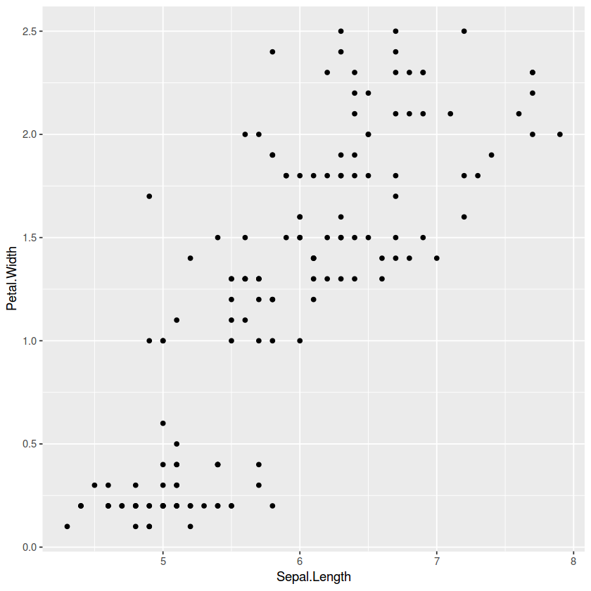
sct_pl_1 <- ggplot(data,aes(x=Sepal.Length,y=Petal.Width))
print(sct_pl_1 + geom_point())
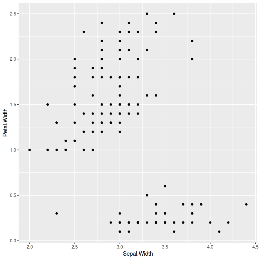
sct_pl_2 <- ggplot(data,aes(x=Sepal.Width,y=Petal.Width))
print(sct_pl_2 + geom_point())
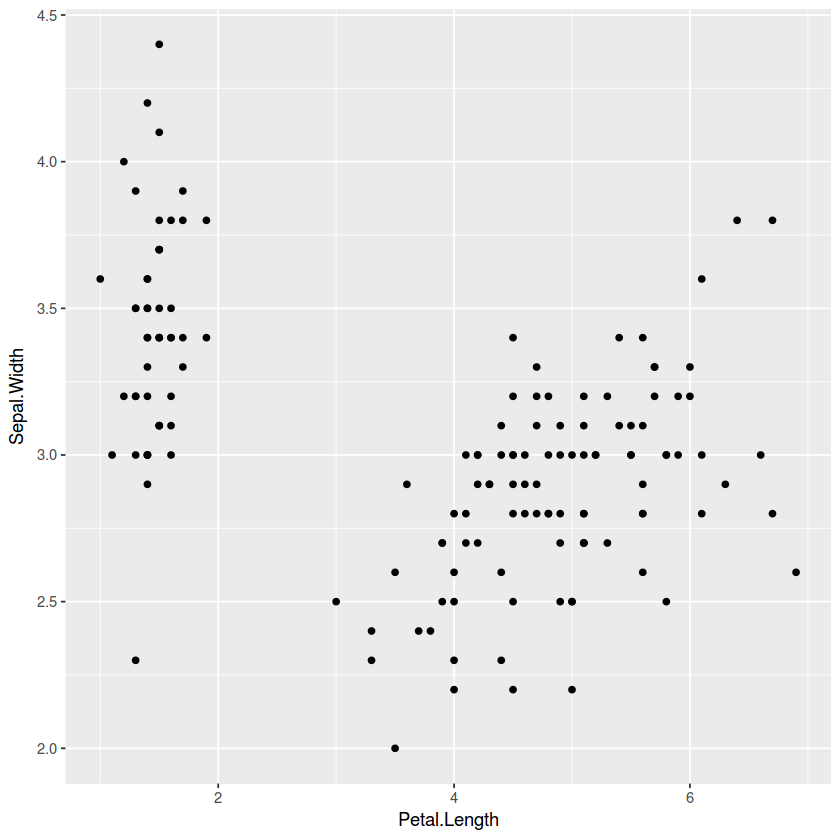
sct_pl_3 <- ggplot(data,aes(x=Petal.Length,y=Sepal.Width))
print(sct_pl_3 + geom_point())
sct_pl_4 <- ggplot(data,aes(x=Petal.Length,y=Petal.Width))
print(sct_pl_4 + geom_point())
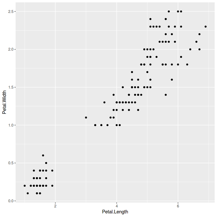
From the previous plots, it seems that the data can be grouped into, minimum, two clusters. One cluster will definitely be easy for K-means to determine, while others might get tricky to define.
The K-means clustering algorithm randomly assigns each observation to a cluster, and finds the centroid of each cluster.
The next process consists of iterating through two steps till the within cluster variation cannot be reduced any further.:
- Reassign data points to the cluster whose centroid is closest.
- Calculate new centroid of each cluster.
the algorithm is already loaded with R, so there is no need for an extra library.
Since this is an unsupervised task, there is no training or testing step, we will go on and try different clustering numbers for our data and visualize the result
K-Means Clustering
# We will try 2 clusters for a start
# For more information, help("kmeans")
two_clusters <- kmeans(data, 2,nstart = 20 )
two_clusters
K-means clustering with 2 clusters of sizes 97, 53

Cluster means:
  Sepal.Length Sepal.Width Petal.Length Petal.Width
1     6.301031    2.886598     4.958763    1.695876
2     5.005660    3.369811     1.560377    0.290566

Clustering vector:
  [1] 2 2 2 2 2 2 2 2 2 2 2 2 2 2 2 2 2 2 2 2 2 2 2 2 2 2 2 2 2 2 2 2 2 2 2 2 2
 [38] 2 2 2 2 2 2 2 2 2 2 2 2 2 1 1 1 1 1 1 1 2 1 1 1 1 1 1 1 1 1 1 1 1 1 1 1 1
 [75] 1 1 1 1 1 1 1 1 1 1 1 1 1 1 1 1 1 1 1 2 1 1 1 1 2 1 1 1 1 1 1 1 1 1 1 1 1
[112] 1 1 1 1 1 1 1 1 1 1 1 1 1 1 1 1 1 1 1 1 1 1 1 1 1 1 1 1 1 1 1 1 1 1 1 1 1
[149] 1 1

Within cluster sum of squares by cluster:
[1] 123.79588  28.55208
 (between_SS / total_SS =  77.6 %)

Available components:

[1] "cluster"      "centers"      "totss"        "withinss"     "tot.withinss"
[6] "betweenss"    "size"         "iter"         "ifault"
three_clusters <- kmeans(data, 3,nstart = 20 )
three_clusters
K-means clustering with 3 clusters of sizes 38, 50, 62

Cluster means:
  Sepal.Length Sepal.Width Petal.Length Petal.Width
1     6.850000    3.073684     5.742105    2.071053
2     5.006000    3.428000     1.462000    0.246000
3     5.901613    2.748387     4.393548    1.433871

Clustering vector:
  [1] 2 2 2 2 2 2 2 2 2 2 2 2 2 2 2 2 2 2 2 2 2 2 2 2 2 2 2 2 2 2 2 2 2 2 2 2 2
 [38] 2 2 2 2 2 2 2 2 2 2 2 2 2 3 3 1 3 3 3 3 3 3 3 3 3 3 3 3 3 3 3 3 3 3 3 3 3
 [75] 3 3 3 1 3 3 3 3 3 3 3 3 3 3 3 3 3 3 3 3 3 3 3 3 3 3 1 3 1 1 1 1 3 1 1 1 1
[112] 1 1 3 3 1 1 1 1 3 1 3 1 3 1 1 3 3 1 1 1 1 1 3 1 1 1 1 3 1 1 1 3 1 1 1 3 1
[149] 1 3

Within cluster sum of squares by cluster:
[1] 23.87947 15.15100 39.82097
 (between_SS / total_SS =  88.4 %)

Available components:

[1] "cluster"      "centers"      "totss"        "withinss"     "tot.withinss"
[6] "betweenss"    "size"         "iter"         "ifault"
Clusters Visualization
# We will load the "cluster" library to visualize clusters
# For installation: install.packages('cluster')
library('cluster')
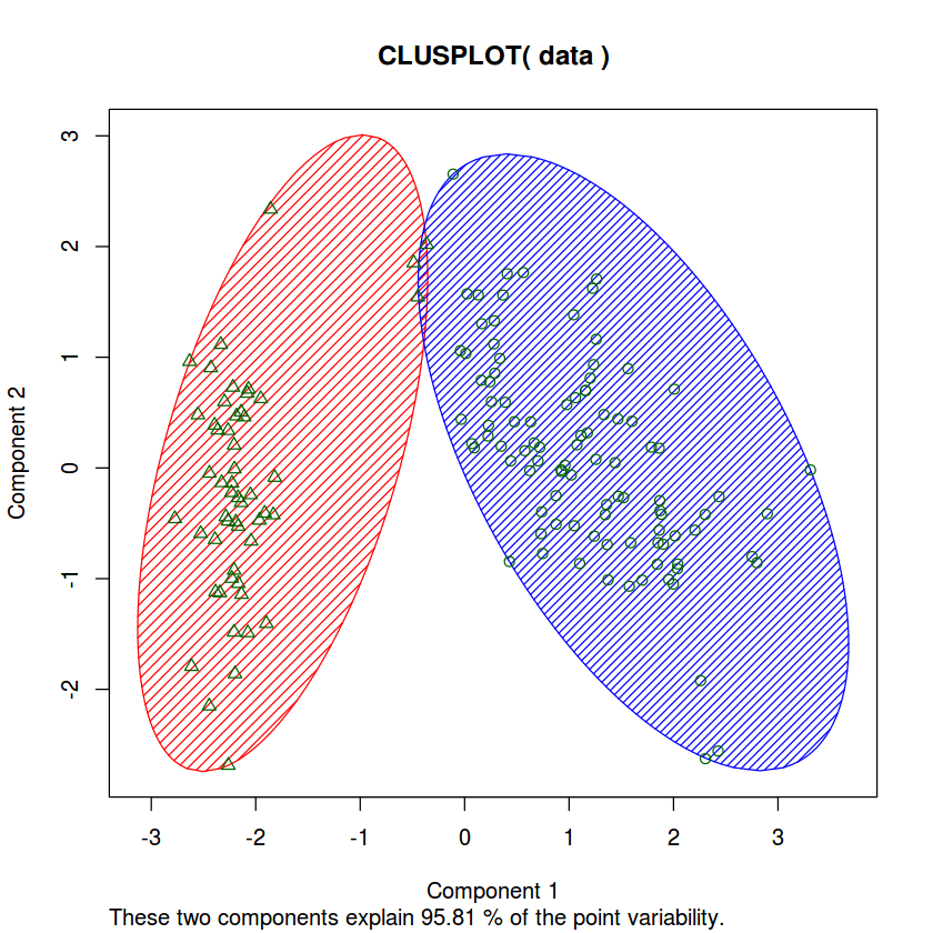
clusplot(data, two_clusters$cluster, color=TRUE, shade=TRUE, labels=0,lines=0, )
clusplot(data, three_clusters$cluster, color=TRUE, shade=TRUE, labels=0,lines=0, )
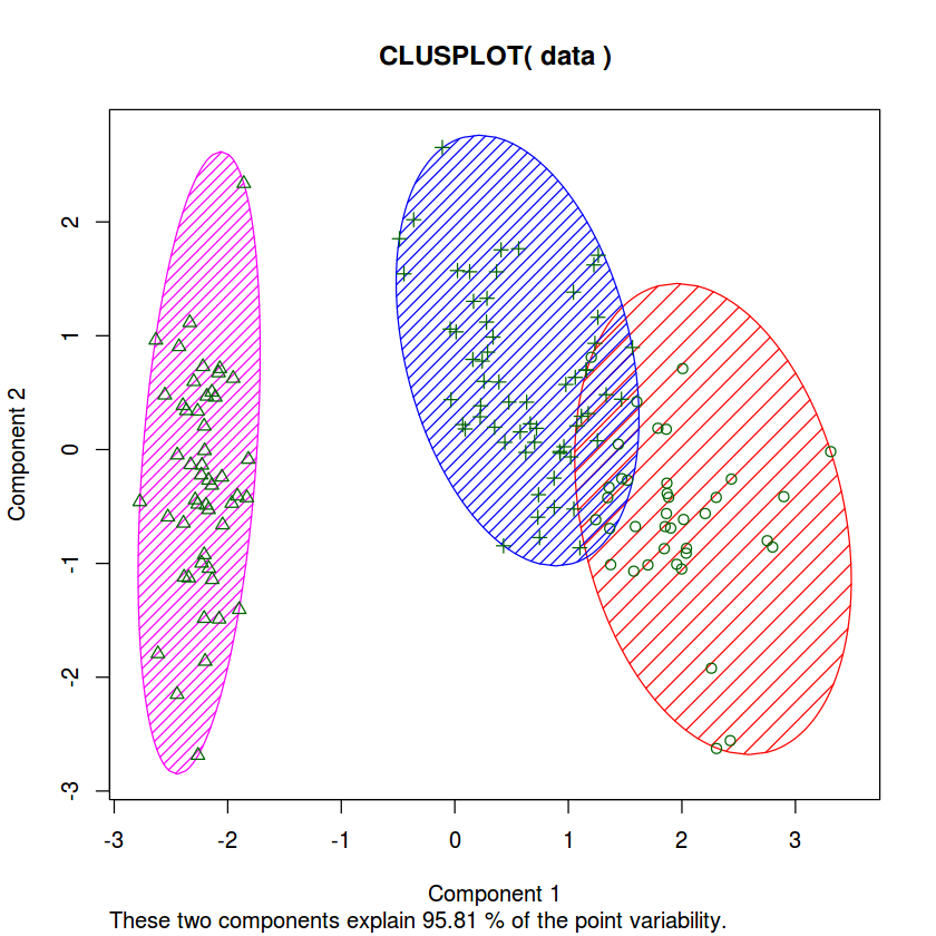
Since we have the luxury of knowing the correct label for each kind of Iris flowers, and just out of curiosity, we will see how the algorithm did with clustering our data.
table(three_clusters$cluster, iris$Species)
    setosa versicolor virginica
  1      0          2        36
  2     50          0         0
  3      0         48        14
As expected, the Setosa was correctly grouped, however, as seen in the previous post, there will always be that overlap between Versicolor and Virginica which explains the misclassification.