Python : Image Recognition With Neural Networks Using TensorFlow

We have been using machine learning methods during the last posts to perform different tasks: classification, regression, clustering and so on. In this post we will begin to talk about deep learning.

Deep learning is an area of machine learning that imitates the workings of the human brain in processing data and creating patterns for use in decision making.

Deep learning is a subset of machine learning in AI that has networks which are capable of unsupervised learning from data that is unstructured or unlabeled.

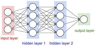
Artificial Neural Networks are inspired by the understanding of the biology of the brain with interconnections between the neurons. In the brain, any neuron can connect to any other neuron within a certain physical distance, however, artificial neural networks have discrete layers, connections, and directions of data propagation.

For image recognition, an image can be chopped up into a bunch of tiles that are inputted into the first layer of the neural network. Then passes the data to a second layer. The second layer does its task, and so on, until the final layer and the final output is produced.

We will train neural networks using TensorFlow which is an open-source software library for numerical computation. More information on it and how it can be installed can be found on the official website.

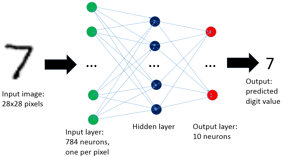
In this post we will try to classify hand written digits from the famous MNIST dataset.

Each row represents black and white images of size 28 x 28 pixels. The features will be the pixel values for each pixel. The value of the pixel is “white” (blank with a 0), or some pixel value.

The goal is to correctly predict what number is written down based on the image data. This type of problem is called Image Recognition and it is a famous use case for deep learning methods.

Getting to know the data

# Import Tensorflow and MINST data
import tensorflow as tf
from tensorflow.examples.tutorials.mnist import input_data
mnist = input_data.read_data_sets("/tmp/data/", one_hot=True)

mnist.train.images[7].shape

(784,)

# we need to get the data
# into (28,28) format for visualization
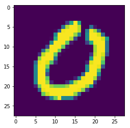
example = mnist.train.images[7].reshape(28,28)

import matplotlib.pyplot as plt
%matplotlib inline
plt.imshow(example)

<matplotlib.image.AxesImage at 0x7f323e1f90b8>

Some parameters need to be adjusted before training our neural network:

Learning Rate

The speed with which a neural network learns is called its learning rate.

In general, we need to find a learning rate that is low enough that the network converges to something useful, but high enough that we don’t have to spend years training it.

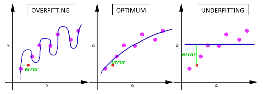
Epochs

An epoch is when an entire dataset is passed forward and backward through the neural network only once. the number of epochs should be chosen carefully because a small number of epochs could lead to under-fitting. On the other hand, a big number will cause over-fitting.

Batch Size

An entire dataset cannot be fed into the neural net at once. So, it should be divided into a number of batches or parts.

learning_rate = 0.001
nb_epochs = 15
batch_size = 100

# Network Parameters
# number of features for the first layer
n_hidden_1 = 256
# number of features for the second layer
n_hidden_2 = 256
# MNIST data input
n_input = 784
# MNIST classes (0-9 digits = 10)
n_classes = 10
n_samples = mnist.train.num_examples

TensorFlow Process

The input data array is sent to the first hidden layer. Then the data will begin to have a random weight attached to it between layers. Then sent to a node to undergo an activation function along with a bias.

Then it will go on to the next hidden layer, and so on until the final output layer. We will just use two hidden layers in this example.

When the data reaches the output layer it needs to be evaluated. Using a loss function (a.k.a. cost function) we can evaluate how many of the classes were correctly predicted.

Then, an optimization function is applied to minimize the cost (lower the error). This is done by adjusting weight values accordingly across the network.

In this example, we will use 2 hidden layers, which use the RELU activation function. It is a very simple rectifier function which essentially either returns x or zero. For our final output layer we will use a linear activation with matrix multiplication.

# TensorFlow Inputs
x = tf.placeholder("float", [None, n_input])
y = tf.placeholder("float", [None, n_classes])

# Weights
weights = {
    'h1': tf.Variable(tf.random_normal([n_input, n_hidden_1])),
    'h2': tf.Variable(tf.random_normal([n_hidden_1, n_hidden_2])),
    'out': tf.Variable(tf.random_normal([n_hidden_2, n_classes]))
}

# Bias
biases = {
    'b1': tf.Variable(tf.random_normal([n_hidden_1])),
    'b2': tf.Variable(tf.random_normal([n_hidden_2])),
    'out': tf.Variable(tf.random_normal([n_classes]))
}

# Twolayer Perceptron
def twolayer_perceptron(x, weights, biases):

    # First hidden layer
    layer_1 = tf.add(tf.matmul(x, weights['h1']), biases['b1'])
    layer_1 = tf.nn.relu(layer_1)

    # Second hidden layer
    layer_2 = tf.add(tf.matmul(layer_1, weights['h2']), biases['b2'])
    layer_2 = tf.nn.relu(layer_2)

    # Last Output layer with linear activation
    out_layer = tf.matmul(layer_2, weights['out']) + biases['out']
    return out_layer

# model def
md = twolayer_perceptron(x, weights, biases)

# cost and optimizer
cost = tf.reduce_mean(tf.nn.softmax_cross_entropy_with_logits(logits=md,labels=y))
optimizer = tf.train.AdamOptimizer(learning_rate=learning_rate).minimize(cost)

# Initializing the variables
init = tf.global_variables_initializer()

Running the Session

if 'session' in locals() and session is not None:
    print('Close interactive session')
    session.close()

# Launch the session
sess = tf.InteractiveSession()

# Intialize all the variables
sess.run(init)

# Training Epochs
for epoch in range(nb_epochs):

    # Starting with cost = 0.0
    avg_cost = 0.0

    # Converting the total number of batches to integer
    total_batch = int(n_samples/batch_size)

    # Looping over all batches
    for i in range(total_batch):

        # Grab the next batch of training data and labels
        batch_x, batch_y = mnist.train.next_batch(batch_size)

        # Feed dictionary for optimization and cost value
        _, c = sess.run([optimizer, cost], feed_dict={x: batch_x, y: batch_y})

        # Compute average loss
        avg_cost += c / total_batch

    print("Epoch: {} cost={:.4f}".format(epoch+1,avg_cost))

print("Model has completed {} Epochs of Training".format(nb_epochs))

Epoch: 1 cost=175.6992
Epoch: 2 cost=39.1834
Epoch: 3 cost=24.8411
Epoch: 4 cost=17.4307
Epoch: 5 cost=12.6881
Epoch: 6 cost=9.4607
Epoch: 7 cost=7.1431
Epoch: 8 cost=5.2480
Epoch: 9 cost=3.8150
Epoch: 10 cost=2.8557
Epoch: 11 cost=2.1296
Epoch: 12 cost=1.6305
Epoch: 13 cost=1.2104
Epoch: 14 cost=1.0198
Epoch: 15 cost=0.8265
Model has completed 15 Epochs of Training

Testing and Evaluating the model

# Testing the model
accurt_preds = tf.equal(tf.argmax(md, 1), tf.argmax(y, 1))

print(accurt_preds[0])

Tensor("strided_slice_1:0", shape=(), dtype=bool)

cast_accurt_preds = tf.cast(acc_preds, "float")

print(cast_accurt_preds)

Tensor("Cast_1:0", shape=(?,), dtype=float32)

accuracy = tf.reduce_mean(cast_accurt_preds)

mnist.test.labels

array([[0., 0., 0., ..., 1., 0., 0.],
       [0., 0., 1., ..., 0., 0., 0.],
       [0., 1., 0., ..., 0., 0., 0.],
       ...,
       [0., 0., 0., ..., 0., 0., 0.],
       [0., 0., 0., ..., 0., 0., 0.],
       [0., 0., 0., ..., 0., 0., 0.]])

mnist.test.images

array([[0., 0., 0., ..., 0., 0., 0.],
       [0., 0., 0., ..., 0., 0., 0.],
       [0., 0., 0., ..., 0., 0., 0.],
       ...,
       [0., 0., 0., ..., 0., 0., 0.],
       [0., 0., 0., ..., 0., 0., 0.],
       [0., 0., 0., ..., 0., 0., 0.]], dtype=float32)

print("Accuracy:", accuracy.eval({x: mnist.test.images, y: mnist.test.labels}))

Accuracy: 0.9475

Final Thoughts

We got 94% accuracy using 15 epochs. Even though this is a good result, running for more training epochs with this data can produce more accuracy that can get to 99%.