
Python : An Unsupervised Learning Task Using K-Means Clustering
In the previous post, we performed a supervised machine learning in order to classify Iris flowers, and did pretty well in predicting the labels (kinds) of flowers. We could evaluate the performance of our model because we had the “species” column with the name of three iris kinds. Now, let´s imagine that we were not given this column and that we wanted to know if there are different kinds of Iris flower based only on the measurements of length and the width of the sepals and petals. Well, this is a called an unsupervised learning.
Unsupervised learning means that there is no class (label) column which we can use to test and evaluate how well a model is performing. So there is no outcome to be predicted, therefore the goal is trying to find patterns in the data to reach a reasonable conclusion.
We will use the K-means clustering algorithm on our Iris data assuming that we do not have the “species” column. We will investigate if data can be grouped into 3 clusters representing the three species of Iris (Iris setosa, Iris virginica and Iris versicolor).
We will use Python in this post, here is the R version. So let´s dive in :).
Preparing the data
import pandas as pd
import seaborn as sns
import matplotlib.pyplot as plt
%matplotlib inline
iris = sns.load_dataset("iris")
data = iris.drop("species",1)
data.head()
| sepal_length | sepal_width | petal_length | petal_width | |
|---|---|---|---|---|
| 0 | 5.1 | 3.5 | 1.4 | 0.2 |
| 1 | 4.9 | 3.0 | 1.4 | 0.2 |
| 2 | 4.7 | 3.2 | 1.3 | 0.2 |
| 3 | 4.6 | 3.1 | 1.5 | 0.2 |
| 4 | 5.0 | 3.6 | 1.4 | 0.2 |
data.describe()
| sepal_length | sepal_width | petal_length | petal_width | |
|---|---|---|---|---|
| count | 150.000000 | 150.000000 | 150.000000 | 150.000000 |
| mean | 5.843333 | 3.057333 | 3.758000 | 1.199333 |
| std | 0.828066 | 0.435866 | 1.765298 | 0.762238 |
| min | 4.300000 | 2.000000 | 1.000000 | 0.100000 |
| 25% | 5.100000 | 2.800000 | 1.600000 | 0.300000 |
| 50% | 5.800000 | 3.000000 | 4.350000 | 1.300000 |
| 75% | 6.400000 | 3.300000 | 5.100000 | 1.800000 |
| max | 7.900000 | 4.400000 | 6.900000 | 2.500000 |
Exploring the Data
Let´s now do some exploratory data analysis to see if we can get an idea about the data. Remember, we assume we don´t know anything about how many clusters (kinds) of flowers we have from the dataset.
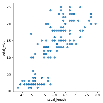
sns.lmplot(x='sepal_length',y='petal_width',data=data,fit_reg=False)
<seaborn.axisgrid.FacetGrid at 0x7fcf98ac0320>
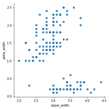
sns.lmplot(x='sepal_width',y='petal_width',data=data,fit_reg=False)
<seaborn.axisgrid.FacetGrid at 0x7fcf98adf4a8>
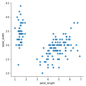
sns.lmplot(x='petal_length',y='sepal_width',data=data,fit_reg=False)
<seaborn.axisgrid.FacetGrid at 0x7fcf90c93550>
sns.lmplot(x='petal_length',y='petal_width',data=iris,fit_reg=False)
<seaborn.axisgrid.FacetGrid at 0x7fcf90b99d30>
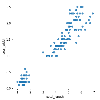
From the previous plots, it seems that the data can be grouped into, minimum, two clusters. One cluster will definitely be easy for K-means to determine, while the others might get tricky to define.
The K-means clustering algorithm randomly assigns each observation to a cluster, and finds the centroid of each cluster.
The next process consists of iterating through two steps till the within cluster variation cannot be reduced any further.:
- Reassign data points to the cluster whose centroid is closest.
- Calculate new centroid of each cluster.
Since this is an unsupervised task, there is no training or testing step, we will go on and try different clustering numbers for our data and visualize the result.
K-Means Clustering
# Importing KMeans from slLearn
from sklearn.cluster import KMeans
# Create an instance of a K Means model with 2 clusters
# Since we are supposed to not know there are 3 species
kmeans_two_md = KMeans(n_clusters=2)
# Fitting the model
kmeans_two_md.fit(data)
KMeans(algorithm='auto', copy_x=True, init='k-means++', max_iter=300,
    n_clusters=2, n_init=10, n_jobs=1, precompute_distances='auto',
    random_state=None, tol=0.0001, verbose=0)
# Cluster center vectors
kmeans_two_md.cluster_centers_
array([[ 5.00566038,  3.36981132,  1.56037736,  0.29056604],
       [ 6.30103093,  2.88659794,  4.95876289,  1.69587629]])
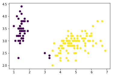
plt.scatter(x='petal_length',y='sepal_width',data=data,c=kmeans_two_md.labels_)
<matplotlib.collections.PathCollection at 0x7fcf8b31a278>
# Create an instance of a K Means model with 3 clusters
kmeans_three_md = KMeans(n_clusters=3)
# Fitting the model
kmeans_three_md.fit(data)
KMeans(algorithm='auto', copy_x=True, init='k-means++', max_iter=300,
    n_clusters=3, n_init=10, n_jobs=1, precompute_distances='auto',
    random_state=None, tol=0.0001, verbose=0)
# Cluster center vectors
kmeans_three_md.cluster_centers_
array([[ 6.85      ,  3.07368421,  5.74210526,  2.07105263],
       [ 5.006     ,  3.428     ,  1.462     ,  0.246     ],
       [ 5.9016129 ,  2.7483871 ,  4.39354839,  1.43387097]])
f, (ax1, ax2) = plt.subplots(1, 2, sharey=True,figsize=(12,6))
iris_map = {'virginica':1,'setosa':2, 'versicolor':3}
ax1.set_title('K Means')
ax1.scatter(x='petal_length',y='sepal_width',data=data,c=kmeans_three_md.labels_)
ax2.set_title("Original")
ax2.scatter(x='petal_length',y='sepal_width',data=iris,c=iris['species'].apply(lambda x: iris_map[x]))
<matplotlib.collections.PathCollection at 0x7fcf8ae20588>
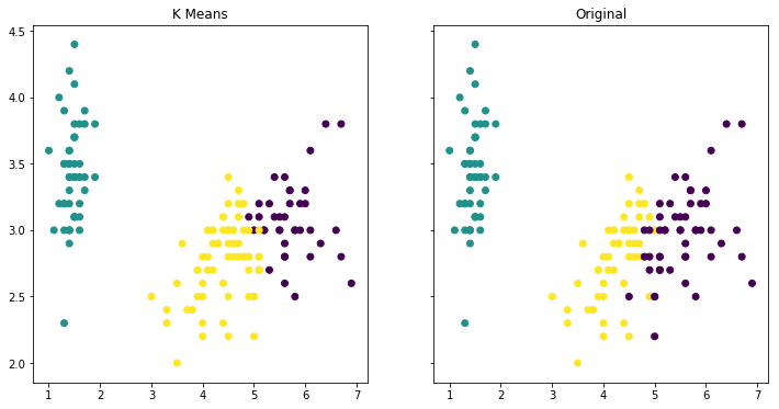
As expected, the Setosa was correctly grouped, however, as seen in the previous post, there will always be that overlap between Versicolor and Virginica which explains the misclassification.