
Python : A Simple Classification Task Using Support Vector Machines
One of the most famous areas of machine learning (ML) is Classification. It consists of identifying to which of a set of categories a new observation belongs. Classification has a broad array of applications, including ad targeting, medical diagnosis and image classification. An example would be detecting if an email is a “spam” or “non-spam”.
Classification is considered an instance of supervised learning. A supervised task learning where a training set of correctly identified observations is available. This consists of analyzing the training data and producing an inferred function, which can be used for mapping new examples. An optimal scenario will allow to correctly determine the class labels to which unseen instances belong.
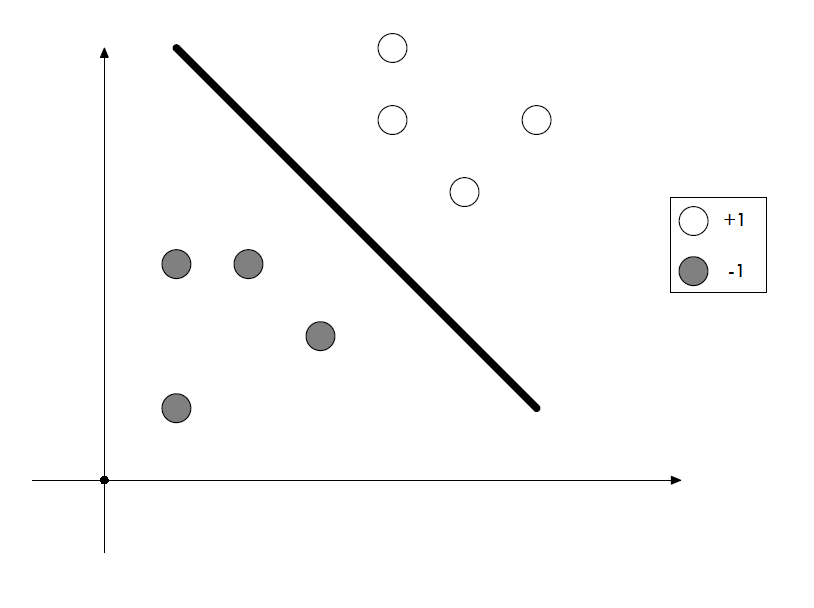
In this post, we will try to classify Iris flowers using Support Vector Machines (SVM) which is a supervised learning method to analyze data and recognize patterns. It is used for both classification and regression analysis.
The Iris flower dataset was introduced by Sir Ronald Fisher back in 1936. It consists of 50 samples from each of three species of Iris:
- Iris Setosa
- Iris Virginica
- Iris Versicolor
Four features were measured from each flower: the length and the width of the sepals and petals, in centimeters.
We will use Python in this post,here is the R version. So let´s start :).
First of all, we will import the necessary packages:
import pandas as pd
# Seaborn is a Python visualization library
# It comes with several datasets, including the iris dataset
import seaborn as sns
%matplotlib inline
# Loading the data
iris = sns.load_dataset("iris")
Getting to know the data
iris.head()
| sepal_length | sepal_width | petal_length | petal_width | species | |
|---|---|---|---|---|---|
| 0 | 5.1 | 3.5 | 1.4 | 0.2 | setosa |
| 1 | 4.9 | 3.0 | 1.4 | 0.2 | setosa |
| 2 | 4.7 | 3.2 | 1.3 | 0.2 | setosa |
| 3 | 4.6 | 3.1 | 1.5 | 0.2 | setosa |
| 4 | 5.0 | 3.6 | 1.4 | 0.2 | setosa |
iris.describe()
| sepal_length | sepal_width | petal_length | petal_width | |
|---|---|---|---|---|
| count | 150.000000 | 150.000000 | 150.000000 | 150.000000 |
| mean | 5.843333 | 3.057333 | 3.758000 | 1.199333 |
| std | 0.828066 | 0.435866 | 1.765298 | 0.762238 |
| min | 4.300000 | 2.000000 | 1.000000 | 0.100000 |
| 25% | 5.100000 | 2.800000 | 1.600000 | 0.300000 |
| 50% | 5.800000 | 3.000000 | 4.350000 | 1.300000 |
| 75% | 6.400000 | 3.300000 | 5.100000 | 1.800000 |
| max | 7.900000 | 4.400000 | 6.900000 | 2.500000 |
iris.isnull().values.any()
False
We can see that the dataset is clear and complete, which means we can move on to the next step.
Exploring the Data
We will visualize data using the Seaborn library. The visualizations will help to get an idea on the separability (degree of classification) across the three species.
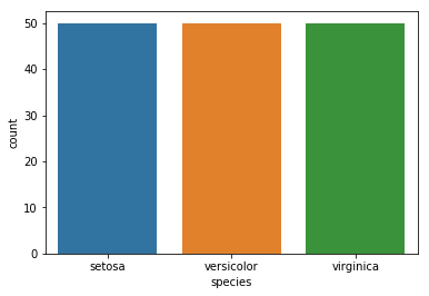
We already know that there are 50 instances per flower kind. So, we are sure there will be no bias factor during the analysis. If we did not know that before hand, a simple countplot can inform us about distribution in the dataset.
sns.countplot(x='species',data=iris)
<matplotlib.axes._subplots.AxesSubplot at 0x7f5678580e48>
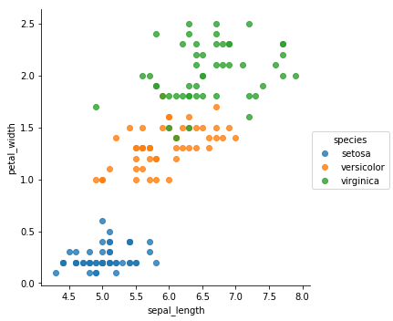
Let´s now explore the different features and see how they contribute to Iris flowers classification.
sns.lmplot(x='sepal_length',y='petal_width',hue="species",data=iris,fit_reg=False)
<seaborn.axisgrid.FacetGrid at 0x7f567859a668>
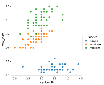
sns.lmplot(x='sepal_width',y='petal_width',hue="species",data=iris,fit_reg=False)
<seaborn.axisgrid.FacetGrid at 0x7f56784ec4a8>
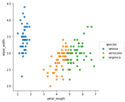
sns.lmplot(x='petal_length',y='sepal_width',hue="species",data=iris,fit_reg=False)
<seaborn.axisgrid.FacetGrid at 0x7f56784638d0>
sns.lmplot(x='petal_length',y='petal_width',hue="species",data=iris,fit_reg=False)
<seaborn.axisgrid.FacetGrid at 0x7f56783d2c18>
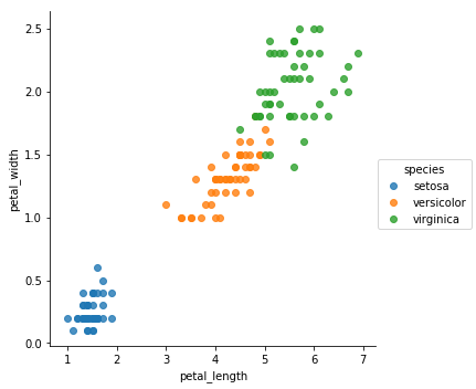
From the previous plots, it appears that the Setosa is very unique compared to the other species. It means that classifying it would be very easy. In the other hand, we can clearly see some overlapping when it comes to Versicolor and Virginica.
Training and Testing the Data
# Y
Y = iris['species']
# X
X = iris.drop('species',axis=1)
# Splitting data into training set and testing set using sklearn
from sklearn.model_selection import train_test_split
X_train, X_test, y_train, y_test = train_test_split(X, Y, test_size=0.33)
# Training the model using Support Vector Machine Classifier (SVC)
from sklearn.svm import SVC
svm_model = SVC()
svm_model.fit(X_train,y_train)
SVC(C=1.0, cache_size=200, class_weight=None, coef0=0.0,
  decision_function_shape='ovr', degree=3, gamma='auto', kernel='rbf',
  max_iter=-1, probability=False, random_state=None, shrinking=True,
  tol=0.001, verbose=False)
# Testing and Evaluating the model
predictions = svm_model.predict(X_test)
from sklearn.metrics import classification_report,confusion_matrix
print(confusion_matrix(y_test,predictions))
[[14  0  0]
 [ 0 16  1]
 [ 0  1 18]]
print(classification_report(y_test,predictions))
             precision    recall  f1-score   support

     setosa       1.00      1.00      1.00        14
 versicolor       0.94      0.94      0.94        17
  virginica       0.95      0.95      0.95        19

avg / total       0.96      0.96      0.96        50
We can clearly see that the model is doing a great job in classifying the Iris flowers, especially the Setosa. For the remaining species, even thought we are predicting the correct label pretty well, we will see if we can do better by performing “Parameter Tuning”
Tuning Parameters and Model Selection
For most ML algorithms, there are some parameters that should be adjusted to make the model more accurate.
One thing should be kept in mind though: we want a model that can be able to predict the correct label for unseen data while doing good with the used data. This means that our model should not fit training data too well (over-fitting), but also, it should not come to the point where it can neither model the training data nor generalize to new data (under-fitting).
A perfect scenario would be to select a model at the sweet spot between under-fitting and over-fitting. This is the ultimate goal of ML, but it is often very difficult to do in practice.
For now, let´s try to try different values for the SVM parameters. There are two parameters that could be adjusted: Cost (C) and Gamma.
The Gamma parameter defines how far the influence of a single training example reaches, with low values meaning ‘far’ and high values meaning ‘close’.
The C parameter trades off misclassification of training examples against simplicity of the decision surface. A low C makes the decision surface smooth, while a high C aims at classifying all training examples correctly.
Instead of trying combinations of parameters one by one and deciding which is the optimal values to choose for the model, we will use GridSearch from Scikitlearn.
GridSearch exhaustively considers all parameter combinations then outputs the settings that achieved the highest score in the validation procedure.
# Gridsearch step
from sklearn.model_selection import GridSearchCV
params_values = {'C': [ 0.1, 10, 100], 'gamma': [1,0.1,0.01,0.001]}
# grid ftting
grds = GridSearchCV(SVC(),params_values)
grds.fit(X_train,y_train)
GridSearchCV(cv=None, error_score='raise',
       estimator=SVC(C=1.0, cache_size=200, class_weight=None, coef0=0.0,
  decision_function_shape='ovr', degree=3, gamma='auto', kernel='rbf',
  max_iter=-1, probability=False, random_state=None, shrinking=True,
  tol=0.001, verbose=False),
       fit_params=None, iid=True, n_jobs=1,
       param_grid={'C': [0.1, 10, 100], 'gamma': [1, 0.1, 0.01, 0.001]},
       pre_dispatch='2*n_jobs', refit=True, return_train_score='warn',
       scoring=None, verbose=0)
We will now use the results for testing and evaluating the model and see if we get a better performance.
new_predictions = grds.predict(X_test)
print(confusion_matrix(y_test,new_predictions))
[[14  0  0]
 [ 0 16  1]
 [ 0  0 19]]
print(classification_report(y_test,new_predictions))
             precision    recall  f1-score   support

     setosa       1.00      1.00      1.00        14
 versicolor       1.00      0.94      0.97        17
  virginica       0.95      1.00      0.97        19

avg / total       0.98      0.98      0.98        50
Final Thoughts
We can see that we got an improvement by tuning the parameters. However, there will always be the overlap between Versicolor and Virginica which explains the misclassification. Anyways, as mentioned earlier, we would like to keep our model capability to generalize to new data in the future, so we will not go further and will settle for this last classifier.